1.1 Fluid :
Fluid is substance that does not permanently resist the distortion. Ideal fluid offers no resistance to change, it is frictionless & incompressible. Compressibility is a measure of the change in volume of a fluid under external forces
The incompressible flow is one where the fluid density is constant, or nearly constant. Liquid flows are generally considered incompressible. If pressure and/or temperature differences are minor enough to make density differences negligible, compressible fluids, such as gases, can experience an incompressible flow. Flows in which the density varies by more than 5 to 10 percent can be considered as compressible flow.
Fluids are liquid, gas and vapors. Study of behavior of fluid is fluid mechanics. Fluid static is fluid at equilibrium state of no shear stress. Fluid dynamics is fluid is in motion relative to other part.
Shear stress is given by Newton’s Law of Viscosity:
\(\tau = \mu \frac{du}{dy}\)Where,
Shear Stress (τ, N/m2): Force per unit area of the shearing plane
Viscosity (µ, Pa-s): It is measure of its resistance to flow
Velocity gradient, du/dy, rate of shear deformation
Kinetic viscosity (ϒ, m2/s): Ratio of viscosity to density
| Pa-s | P | cP |
|---|---|---|
| 1 | 10 | 1000 |
| 0.1 | 1 | 100 |
| 10-3 | 0.01 | 1 |
1.2 Fluid Properties :
The following are the properties of fluids. They are density, viscosity, molecular weight and specific heat.
Density (kg/m3) is weight per volume of fluid. The gas density (kg/m3) is depends on pressure and temperature and given by PM/RT. The density of the mixture is sum of product of mass fraction and density of each component in mixture.
Molecular weight (kg/mole) is mass per unit mole. Average molecular weight the mixture is sum of product of mass fraction and molecular weight of each component in mixture.
Viscosity (µ, Pa-s) is measure of its resistance to flow. The relation is given by Newton’s law of viscosity.
Kinetic viscosity (ϒ, m2/s) is the ratio of viscosity to density.
Specific heat capacity (J/kg·K) is the energy required to increase temperature of material of a certain mass by 1°C. Cp is heat capacity at constant pressure. Cv is heat capacity at constant volume. Constant volume indicates that there is no change in volume. Therefore the only change in the system is internal energy of the system, due to the addition of heat.
1.3 Newtonian and Non-Newtonian fluids :
Power Law: Ostwald de waele equation:
\(\tau = k \left( \frac{du}{dy} \right)^n\)Based on values of n fluids are classified as
- Newtonian (k= µ, n=1) fluid. Most gas and liquids are Newtonian
- Dilatant (n > 1). Example is starch suspension in water
- Pseudo-plastic (n < 1 ) : Examples are Blood, polymer solution and mud
- Bingham plastic (require initial shear stress to flow). Example are Jelley and toothpaste Viscosity can change with time
- Thixotropic: Apparent viscosity may decrease with time under shear stress but recover when the shear stress is removed, paint ink
- Rheopectic: When viscosity increases with time under an constant shear rate, Bentonite sols
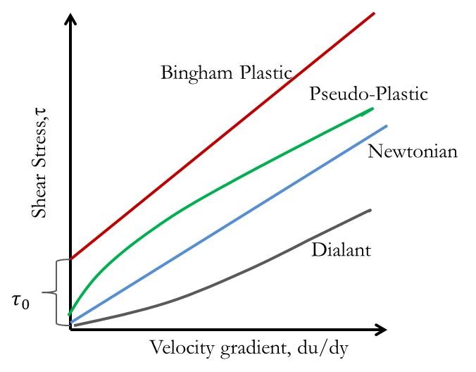
Type of fluids is shown in Figure 1.
1.4 Laminar and Turbulent Flow :
When fluid flows through a pipe, the velocity at point perpendicular to direction of flow is not uniform. The net velocity at the wall is negligible due to wall friction resistance. Velocity increase as we move away from wall and velocity is the maximum at center. If fluid is frictionless and conditions of slip exist at pipe wall, the velocity becomes uniform throughout the cross section of the pipe and velocity profile becomes flat called plug flow.
Laminar flow: At lower velocities fluid particles move smoothly, parallel everywhere. Since fluid moves in a laminated form or layers, this is called laminar flow. The flow is decided by Reynolds number.
\( Re = \frac{DV\rho}{\mu} \)Laminar flow is when Reynold Number < 2100
Turbulent Flow: At higher velocities fluid particles move along very irregular paths, causing an exchange of momentum between the fluid particles (portions). Reynold Number > 2100, then flow is turbulent flow.
The fractional loss in laminar flow varies proportional to flow and in case of turbulent flow fractional loss is proportional to velocity power 1.7 to 2.
1.5 Macroscopic and Microscopic Balances :
The conservation of mass, conservation of momentum and conservation of energy are regarded as fundamentals in fluid dynamics.
Mass balance (Continuity Equation):
The mass of fluid entering and leaving the tube in unit time is equal.
\( m = \rho u A = \text{Constant} \) \( m = \rho_a u_a A_a = \rho_b u_b A_b \) \( u_a A_a = u_b A_b \)For constant density,
Volumetric flow (Q) is product of average velocity (u) and cross section area (A). The average mass velocity is G = \( \rho V \).
For steady flows with multiple inlets and/or outlets through fixed control volumes, the sum of Inlet weight flow rates are equal to the outlet mass flow rates.
For incompressible fluids, mass input equal to mass output in steady as well as unsteady state.
Momentum Balance
The sum of all forces acting on the fluid equal to the increase in the time rate of momentum of flowing fluid. The sum of forces acting in x direction equals the difference between the momentum leaving with fluid per unit time and that brought in per unit time by fluid.
Momentum Balance equation
\( \sum F = M_b - M_a \)Momentum is product of mass flow rate m and velocity u, M=mV
\( \sum F = m(\beta_b V_b - \beta_a V_a) \)β factor is for averaging velocity at inlet and outlet surface. For uniform velocity β is one.
For one dimensional flow in x direction, equation can written as
\( \sum F = p_a A_a - p_b A_b + F_W - F_g \)\(p_a\) and \(p_b\) are inlet and outlet pressures. \(A_a\) and \(A_b\) are inlet and outlet cross section areas
\(F_W\) is net force of wall of channel on fluid
\(F_g\) is component force of gravity.
1.6 Bernoulli’s Theorem :
Mechanical energy balance for steady flow is given by Bernoulli’s theorem. When given elements of a moving fluid undergo expansion, it does mechanical work. This work must be expended on the fluid immediately ahead of it, but fluid elements in question also pick up an equivalent amount of mechanical energy at expense of the internal energy of fluid or externally derived heat. Granting reversibility of expansion, this self-expansion work PdV is to be included in a mechanical balance. When the fluid flows from ‘A’ to ‘B’, some of the energy available at ‘A’ is converted into frictional heat and unavailable at ‘B’, Let ‘F’ J/kg friction loss.
Where,
Total Energy Balance for steady flow
The total energy content (head) of a fluid in motion has following components. Consider unit mass of fluid and neglect changes in surface energy, magnetic energy, etc.
The total head (energy) at any point in a fluid system is the sum of the potential, static, and velocity heads, besides its internal energy.
After the system has reached the steady state, mass input equal to mass output. If loss of energy is neglected between the points A and B, the energy input equal to energy output
\( E_A + Z_A g + \frac{P_A}{\rho_A} + \frac{u_A^2}{2} = E_B + Z_B g + \frac{P_B}{\rho_B} + \frac{u_B^2}{2} \)Internal energy (EA): Amount of internal energy EJ/kg that is attributable to the physical state of the fluid
Potential head (Zg): It is the vertical distance above reference level which is taken as zero.
Pressure Head (P/\(\rho\)): It is the pressure exerted by the fluid against the wall of the pipe at the point under consideration.
Velocity Head \( \frac{u_A^2}{2} \) : It is the head through which the fluid would have to fall to acquire the velocity that exists at the point in question. Since the fluid is in motion at an average velocity of u m/s, 1kg of fluid will have a kinetic energy equal to ( u2 /2) J/kg. This head depends only upon the velocity of fluid.
If Ws be the energy in J/kg added to the system by means of a pump and Q J/Kg is the net heat absorbed from the surroundings, the principle of conservation of energy gives
\( E_A + Z_A g + \frac{P_A}{\rho_A} + \frac{u_A^2}{2} + Q - w_s = E_B + Z_B g + \frac{P_B}{\rho_B} + \frac{u_B^2}{2} \)The total energy balance eqution(4.22) may also written as
\( Q - w_s = \Delta E + \Delta Z g + \Delta \left( \frac{u^2}{2} \right) \)When \(\Delta\) denotes a finite change in the quantities.
Fluid Head
If a vertical tube upon to the atmosphere at one end is attached to a pipeline carrying a liquid under pressure, the liquid will rise in the tube. It will continue to raise until its weight in the tube produces enough pressure at the bottom to balance the pressure in the pipe at a section where the tube is connected. The plane of the connection opening is parallel to the direction of liquid flow. If P be the pressure of the fluid at a point under consideration, Po be the atmospheric pressure, and h be the height of the liquid in the tube,
\( P = P_0 + h \rho g \) \( h = \frac{\Delta P}{\rho g} \)or
Where, \(\Delta\)P=P-P0 = Guage pressure,
This height h of the fluid is termed as the fluid head. It represent the energy per unit weight of the fluid and has dimensions of the length. \(\Delta\)P/\(\rho\), og gh represent energy per unit mass of the fluid.
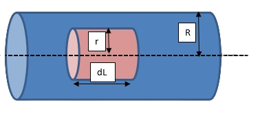
1.7 Hagen – Poiseuille Equation :
Consider a tube-shaped element of fluid, concentric with axis of tube of radius ‘r’ and length ‘dL’. Steady flow of Newtonian fluid of constant density in fully developed flow through a horizontal circular tube under influence of pressure drop dP across pipe.
The forces acting on fluid element are the normal pressure over the ends and shear forces over the curved sides. For steady flow, the forces caused by pressure drop must be balanced by the viscous forces at the boundary of cylindrical element.
The viscosity equation and shear stress relation are used for deriving Hagen-Poiseuille equation.
- Shear Stress
Consider element of length “dL” and radius “r”.
Momentum Balance equation
\( \sum F = \frac{m}{g_c} (\beta_b V_b - \beta_a V_a) \) \( \sum F = 0 \quad \text{As} \quad (\beta_b = \beta_a \quad \text{and} \quad V_b = V_a) \) \( \sum F = P_a A_a - P_b A_b + F_W - F_g \) \( A_a = A_b = \pi r^2 \) \( F_w = F_s = (2\pi r \, dL) \tau \) \( P_b = P_a + dP \)Hence
\( \sum F = P_a \pi r^2 - (P_a + dP) \pi r^2 + (2\pi r \, dL) \tau = 0 \) \( \frac{dP}{dL} + \frac{2\tau}{r} = 0 \)At wall of the pipe
\( \frac{dP}{dL} + \frac{2\tau_w}{R} = 0 \) \( \frac{\tau}{r} = \frac{\tau_w}{R} \) \( \tau = \frac{r \tau_w}{R} \)Newton’s Viscosity equation is
\( \frac{du}{dr} = -\frac{\tau}{\mu} = -\frac{r \tau_w}{\mu R} \) \( \int_0^u du = -\frac{\tau_w}{\mu R} \int_R^r r \, dr \) \( u = \frac{\tau_w}{2\mu R} (R^2 - r^2) \) \( u_{max} = \frac{\tau_w R}{2\mu} \quad \text{(at pipe center where } r=0) \) \( \frac{u}{u_{max}} = 1 - \left(\frac{r}{R}\right)^2 \)The average velocity
\( V = \frac{m}{\rho A} = \frac{1}{A} \int_{0}^{R} u \, dA \)The cross-sectional area \( dA = 2\pi r \, dr \)
\( V = \frac{1}{\pi R^2} \int_0^R \frac{\tau_w}{2\mu R} (R^2 - r^2) \, 2\pi r \, dr \) \( V = \frac{\tau_w}{\mu R^3} \int_0^R (R^2 - r^2) \, r \, dr \) \( V = \frac{\tau_w R}{4\mu} \) \( \frac{V}{u_{max}} = 0.5 \)Friction Factor and Wall shear:
\( \tau_w = \frac{dP}{dL} \cdot \frac{R}{2} \) \( V = \frac{R}{4\mu} \cdot \frac{dP}{dL} \cdot \frac{R}{2} \) \( V = \frac{D^2}{32\mu} \left( \frac{dP}{dL} \right) \) \( \frac{dP}{dL} = \frac{32 \mu V}{D^2} \)This is called Hagen-Poiseuille equation.
Fanning Equation:
The pressure drop (in Pa) due to fraction in a pipe can be calculated using fanning equation given below:
\( -\Delta P_f = \frac{2 f \rho V^2 L}{D} \)Frication Factor:
Commonly useful in turbulent flow. It is defined as the ratio of the wall stress to the product of density and the velocity head (V2/2).
\( f = \frac{2\tau_w}{\rho V^2} \) \( f = \frac{2}{\rho V^2} \cdot \frac{4\mu V}{R} \) \( f = \frac{16\mu}{D V \rho} \) \( f = \frac{16}{Re} \)In case of Turbulent flow through a smooth pipe, friction factor is function of Reynold number only and given by
\( f = 0.079 \, Re^{-1/4} \)And
\( \frac{1}{\sqrt{f}} = 4 \log(Re \sqrt{f}) - 0.4 \)Turbulent flow through a rough pipe, friction factor is function of Reynold number and the relative roughness and given by
\( \frac{1}{\sqrt{f}} = -4 \log\left(\frac{e}{3.7d} + \left(\frac{6.81}{Re}\right)^{0.9}\right) \)And
\( \frac{1}{\sqrt{f}} = 3.48 - 4 \log\left(\frac{2e}{d} + \frac{9.35}{Re\sqrt{f}}\right) \)